A practical iOS app identifying poison oak.

Poizon Plants

Poizon Plants

Intro/Motivation

I have gotten poison oak multiple times. While exposure to the oil found on the plant will not cause an allergic reaction for everyone, the fact remains it’s not fun. Also, it should be noted that while some people definitely do not have an allergic reaction, there is no proof that you won’t develop an allergic reaction over time with continued exposure, according to the American Osteopathic College of Dermatology and other sources. Basically, no one is really safe.

Of course, if you don’t live on the West Coast, all of this might not matter too much. While Urushiol (the oil on poison oak causing the allergic reaction) can be found in plants all over the world, it seems to really love the North American West Coast. Those of us living in California or Oregon for more than a few years are likely familiar with, or at least have heard of, poison oak. But even people native to California (much less one of the millions of tourists) have trouble identifying the plant if it’s not in its signature glowing, oily red. It seems like a good use-case for computer vision.

Given that mobile phones are ubiquitous even when out enjoying nature, creating a poison oak app seemed like a useful project and learning opportunity.

Side note: I had no interest in duplicating effort for something that already had a solution, so I did a little research to see if there were any existing solutions for this niche personal challenge. Interestingly enough, there were already a few apps on the iOS store that were simple classification apps like the one I proposed.

Cold-Start Problem

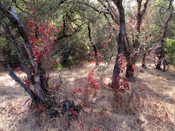
As with any supervised learning challenge, it is critical to get a good source of labeled data. Perhaps the obvious place to start for poison oak was Google Images. Using Chrome extension here, I was able to download large quantities of images.

Semantics of the search were somewhat important (“poison oak”, “poison oak bush”, “poison oak autumn”, etc.), so I focused on making searches that got images of the plant under different seasons. The thought here being to capture as much heterogeneity of poison oak as possible for users of the app. Unsurprisingly, this is the first place where the data revealed its bias since the major season captured for poison oak seemed to be when it was at its most obvious: red or orangish-red starting end of summer. But this is for poison oak during the later half of the year and not even necessarily when it’s at its oiliest.

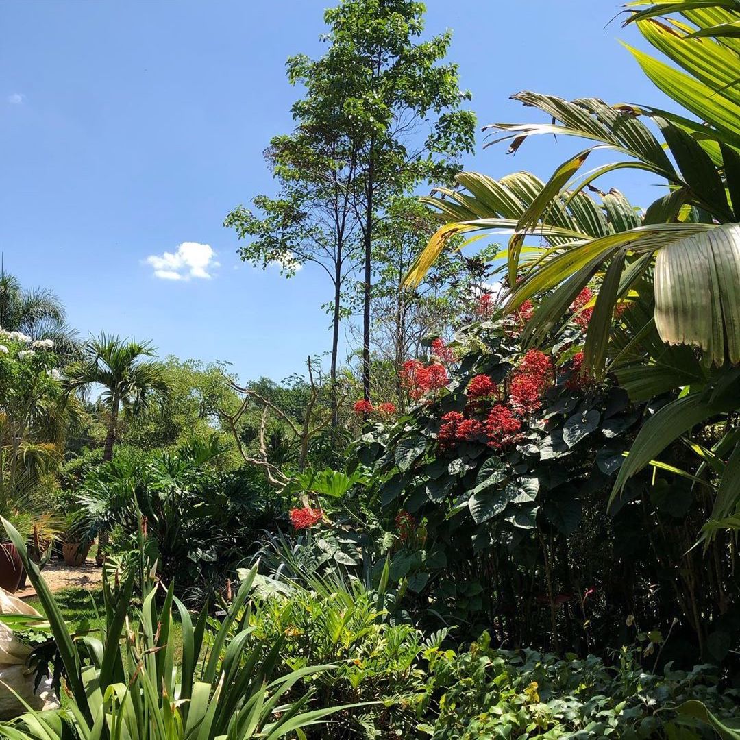
For the “not poison” images, I tried to cover a broad flora that might exist geographically with poison oak and especially on plants whose leaves I thought would confuse the average hiker. This initial dataset netted me about 3k images in total after cleaning out the expected garbage images (cartoons images, stock photo images with watermarks, etc.). Since transfer learning is available, this was a great start and stage to baseline model performance.

To obtain a preliminary understanding of the signal present in the dataset, I implemented a Resnet50 on an 80/20 random split of the data. With minor tuning, I achieved a validation accuracy of over 98%. However, this result appeared suspiciously ideal and indicated a strong presence of bias in the dataset. I suspect that the image data obtained from Google Images may have been generated by a model similar to the one I used for training. Minor differences in data cleaning and algorithms may be responsible for the suboptimal performance, preventing me from achieving 100% accuracy with the model trained on the Google Images.

Of course, the only solution to poor data is get more data. And hopefully that captures more variety for the use-case your modeling for. The benefit of acquiring data this way is that I would be:

1) Labeling on the go and would have more intuition what my model was and wasn’t understanding well.
2) Refining the concept-space of what constituted a reasonable recognition of an image containing poison oak since this could include multiple plants.
3) Have a reason to go on more hikes.

Object Detections Vs Classification

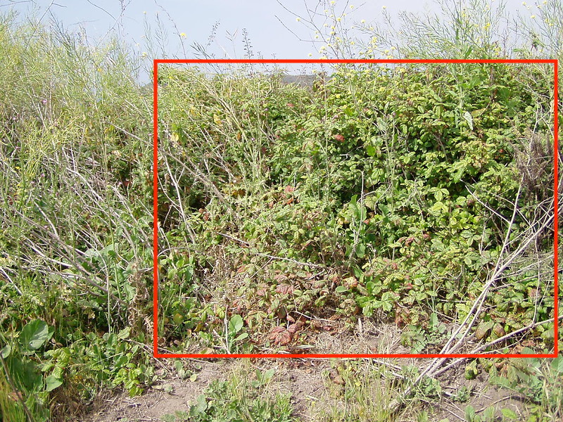
The question arises as to why we refrain from treating this issue strictly as an object detection problem. In an ideal scenario, you would draw a bounding box encapsulating the identified leaf or plant. However, anchoring the project in a practical use-case: an individual equipped with a cell-phone who wants to maintain their distance from the plant in question. As they incrementally approaches, their certainty concerning the classification converges.

Labeling Process

There is a growing demand for quality labeling services. Perhaps the most well known is Mechancial Turk which provides relatively inexpensive labeling service. The challenge here is finding a domain experts which in my case relied on (most likely) utilizing, possibly, non-Californians to decide if a plant was poison oak or not. For an in-house approach services such as LabelBox and Spacy Prodigy provide a great improvement on the efficiency of human labeling. While I’ve had great experiences with Prodigy for NLP projects, since LabelBox provides a limited free access, I utilized their product. Regardless, it’s a tedious process.

Again, I hand-labeled 8000 images that I took with my iphone 7 plus!

Choice of Cut-off Probability

This is a choice which I’ve seen discussed very rarely for a binary classification problem (at least in workshops/tutorials/books). It can have great practical implications for the end-user. Generally you assume the cut-off for a binary classifier at 50/50 for deciding whether to bin the output of the softmax as a 1 or 0. I chose to model the app as a degree of certainty that a given image was poison oak based on feedback from different people I had test the app out. In this case, binning the probabilities into categories such as “possibly poison oak”, “definitely poison oak”, etc. provided better intuition to the user that a 60% vs a 80% probability.

iOS App

App Starting point: Creating an image classifier
Adds on app: Admob and Firebase

Modeling

While initial base-lining of model was quit easy with Apple’s CoreML, it quickly became obvious that the developer-friendly approach to ML wasn’t going to cut it for my self-assigned project. It was a great generalizer and got me 0-60 super quick.

Training

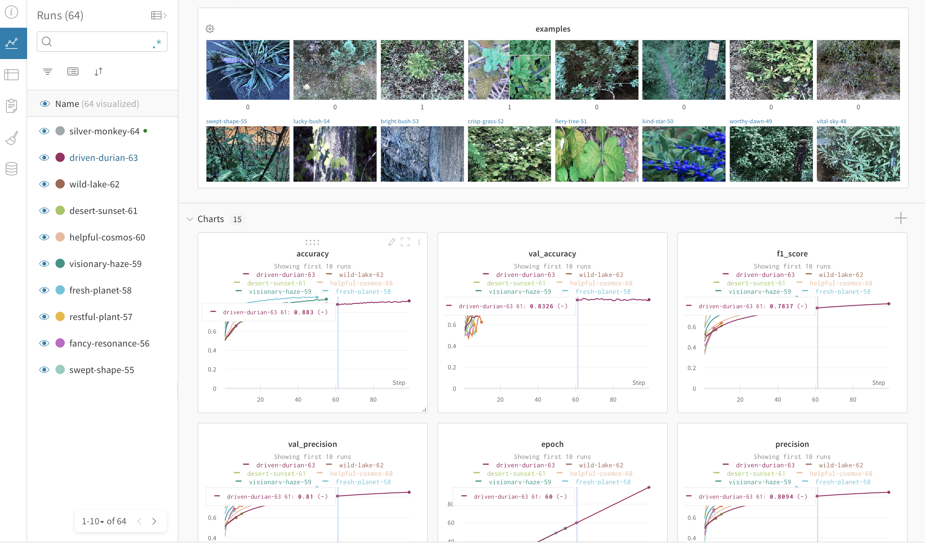
Model Tracking: Utilization of Weights & Biases (wandb.com) was very useful when iterating over different models. It even has an image viewer so that you can peek at how you model is predicting example images while it is training.Wandb Hyper-parameter Sweeps was also very helpful in reducing manual rerunning of hyperparameters.

Contextual image information may often be a confounder.

Choice of architecture:: Due to wanting to have a very controlled way of dealing with outliers, i.e. more distant pictures of a bush of poison oak it was necessary to use both dropout and L2 regularization (Here is a good blog post on this topic). L2 was a reasonable choice for regularization since I wanted to smooth more for those outliers (as opposed to L1 which does not penalize as strongly). The reason for this is in the figure below:
- We don’t particularly care this image has a probability of 92% vs 99%
- We DO care if THIS image has a probability of 60% vs 5%:

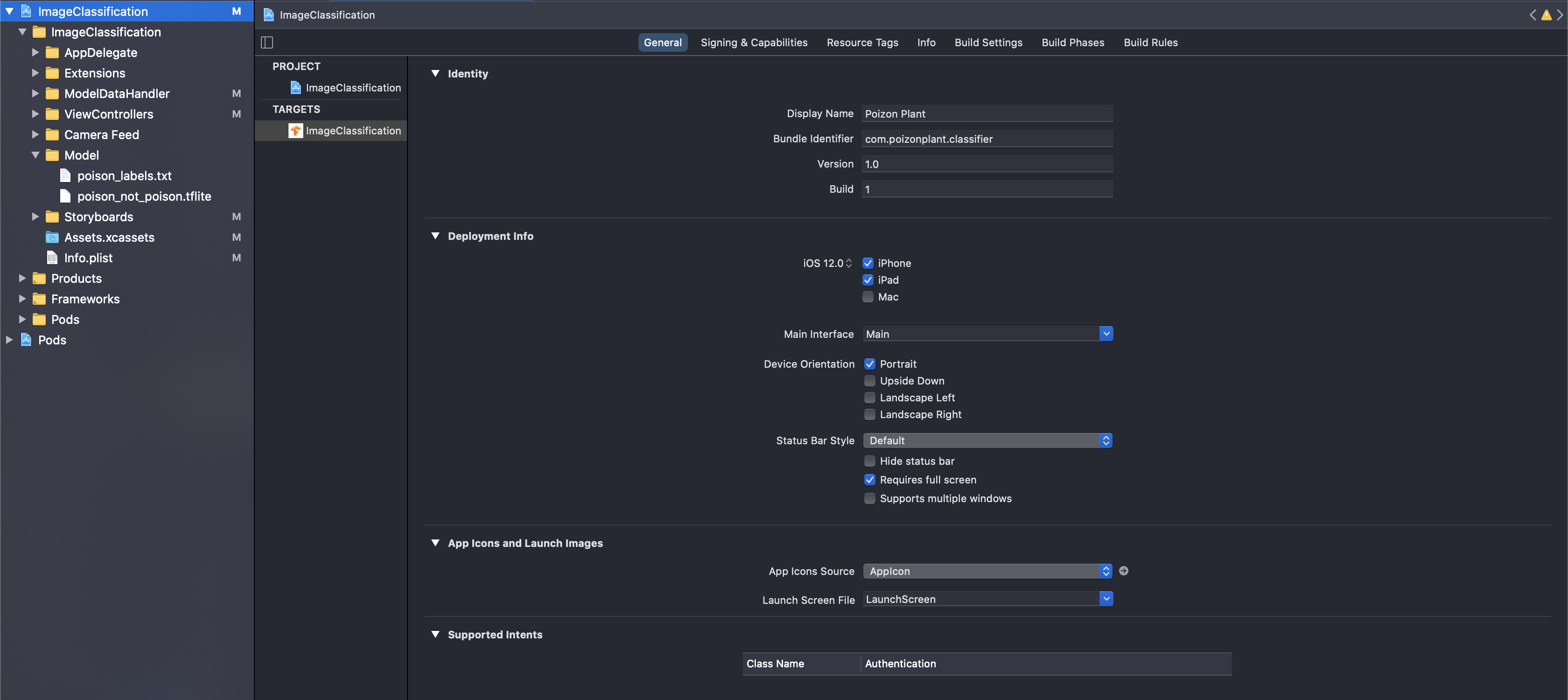
Tayloring model for mobile platform (Converting Tensorflow to TF-Lite)

Why:
- CoreML is not as well supported with documentation etc for complex ML training
- TF-Lite could also easily be used on Android devices (or pretty much anywhere else for that matter)
- Optimizations are offered for TF Lite:
  - Default
  - Latency
  - Size However with my testing (TF V2.3.0), there was a significant (~5%) drop in F1 when optimizing for Latency or Size and not a significant change in user experience.

Convert Keras trained model to TF-lite

# TF: v2.3.0
# Python: v3.8.2

from tensorflow.keras.models import load_model
from tensorflow.lite.TFLiteConverter import from_keras_model

# Load model (I had saved as a .model file and it worked fine)
model = load_model(model_path, custom_objects=dependencies,compile=True)

converter = tf.lite.TFLiteConverter.from_keras_model(model)

# Set True to optimize model for speed
if False:
    print('[INFO] Optimizing TF Lite model')
    converter.optimizations = [tf.lite.Optimize.OPTIMIZE_FOR_SPEED] 
tflite_model = converter.convert()

With my testing, the optimized models did not significantly (even on my dated iPhone 8 plus) change the user experience. The f1-score did significantly drop a few points however, and this was enough for me to use the default settings in TF Lite. I assume on much smaller IOT devices latency and size would greatly outweigh relatively small metric gains from the default.

Save model for use in iOS

import pathlib

# Write model to file
tflite_model_file = pathlib.Path('./poison_not_poison.tflite')
tflite_model_file.write_bytes(tflite_model)

# Write labels to file
labels = ['is_poison','not_poison']

with open('poison_labels.txt','w') as f:
    f.write('\n'.join(labels))

Drop model in iOS app

Other Training Lessons Learned

Initially, I made all layers trainable which resulted in a extremely spiky, but generally decreasing validation loss but only after huge number of 250 epochs. After running some experiments, I found a much steadier decrease of validation loss at training only the last 20 layers which resulted in a smoother convergence and higher overall accuracy. I also experimented with different optimizers, including Adam and SGD, and found that Adam yielded the best results. In addition, I utilized data augmentation techniques such as random rotations and flips to further improve the model’s robustness. Finally, I fine-tuned the hyperparameters of the model, such as the learning rate and batch size, to achieve the best possible performance.
Choice of object detection vs classification task When thinking about how to make the app practical for hikers vs what was practical for modeling, it seemed like there were 2 choices: focus on the object detection task or a classification task.

Practically speaking, it seems more useful that a person would pull out their phone and sweep the camera over a range of plants. Looking ahead, this would involve a lot of manual labeling of bounding boxes and too much work. The project could always be easily extended to include this scope also. So classification it was.

Getting to > 90% F1 score This goal was set both for practical reasons (having a classifier app that was a satisfying product), as well as a mental milestone for “I understand training an image classifier”. There is potentially a lot of learning to be had between an 87% F1 score that I struggled with for a while and 90% F1-score that I finally achieved. Achieving a >90% F1 score was a critical goal for developing a high-quality image classifier app, as well as a personal milestone for my understanding of training such a model. The journey from struggling with an 87% F1 score to finally hitting 90% taught me a lot about the learning potential between these two points.
It was particularly important to optimize on the 299x299 image size used by iOS during model development for performance, compatibility with the iOS platform and consistent testing.
Focus on your highest-loss images to understand true performance This was useful both for cleaning bad/poor quality images as well as finding areas where potentially you might need to break out a new class, e.g. “Unknown bush”
Think your data is well-labeled? Think again…and again:
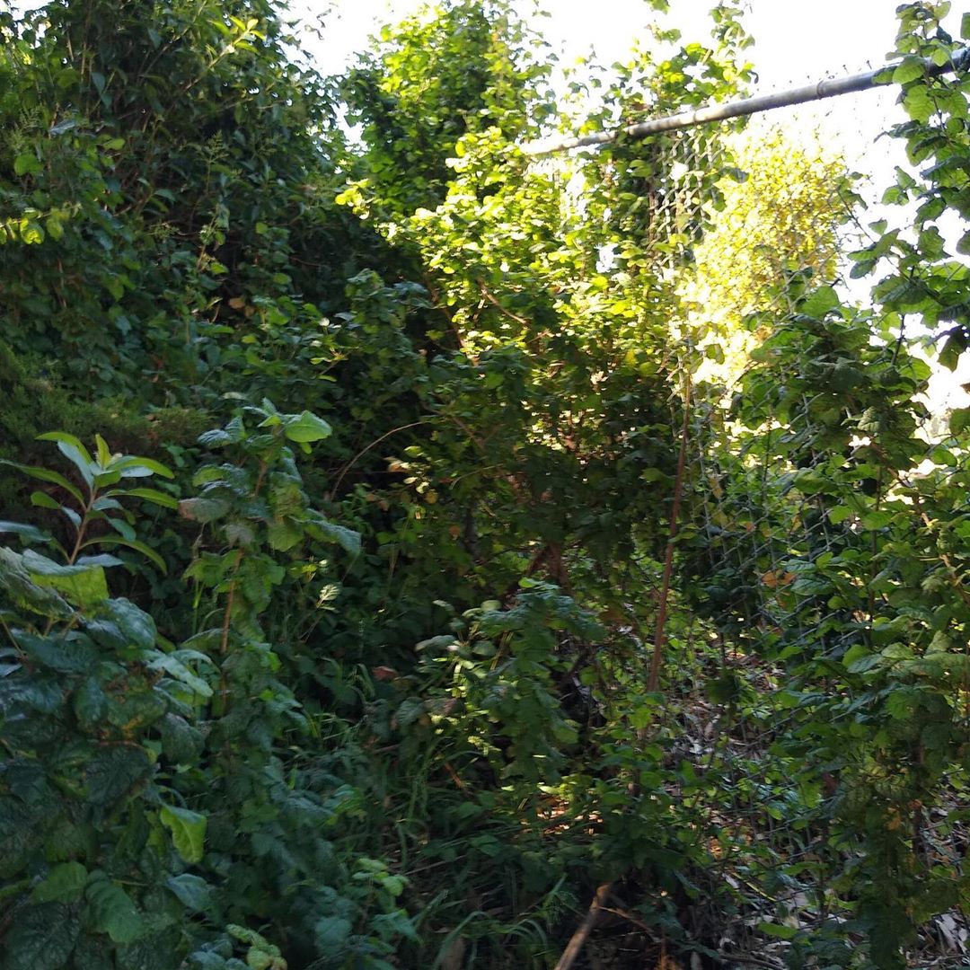
- Despite having gone through and labeled, by hand, thousands of images, examining images with top log-loss showed the my human error. I think one reason for this is during the labeling process, I had additional context for “yes this is poison oak” due to having walked by a large bush of poison oak already. When looking only at the photo that was taken with no additional context, which is what the neural net is doing, it was not clear to my human eye.
How do you know when your data is enough? For the practicality of my problem, where a region captured with a phone camera “may contain poison oak”, it was not immediately clear if I had taken pictures with sufficient variation. An example of when this issue first surfaced was when a reddish plant, which was not poison oak, caused trouble for the algorithm. This presented a bit of a challenge because while red is a strong indicator (for both humans and neural nets) for identifying sumac plants, it is not a definitive rule for identifying poison oak.”

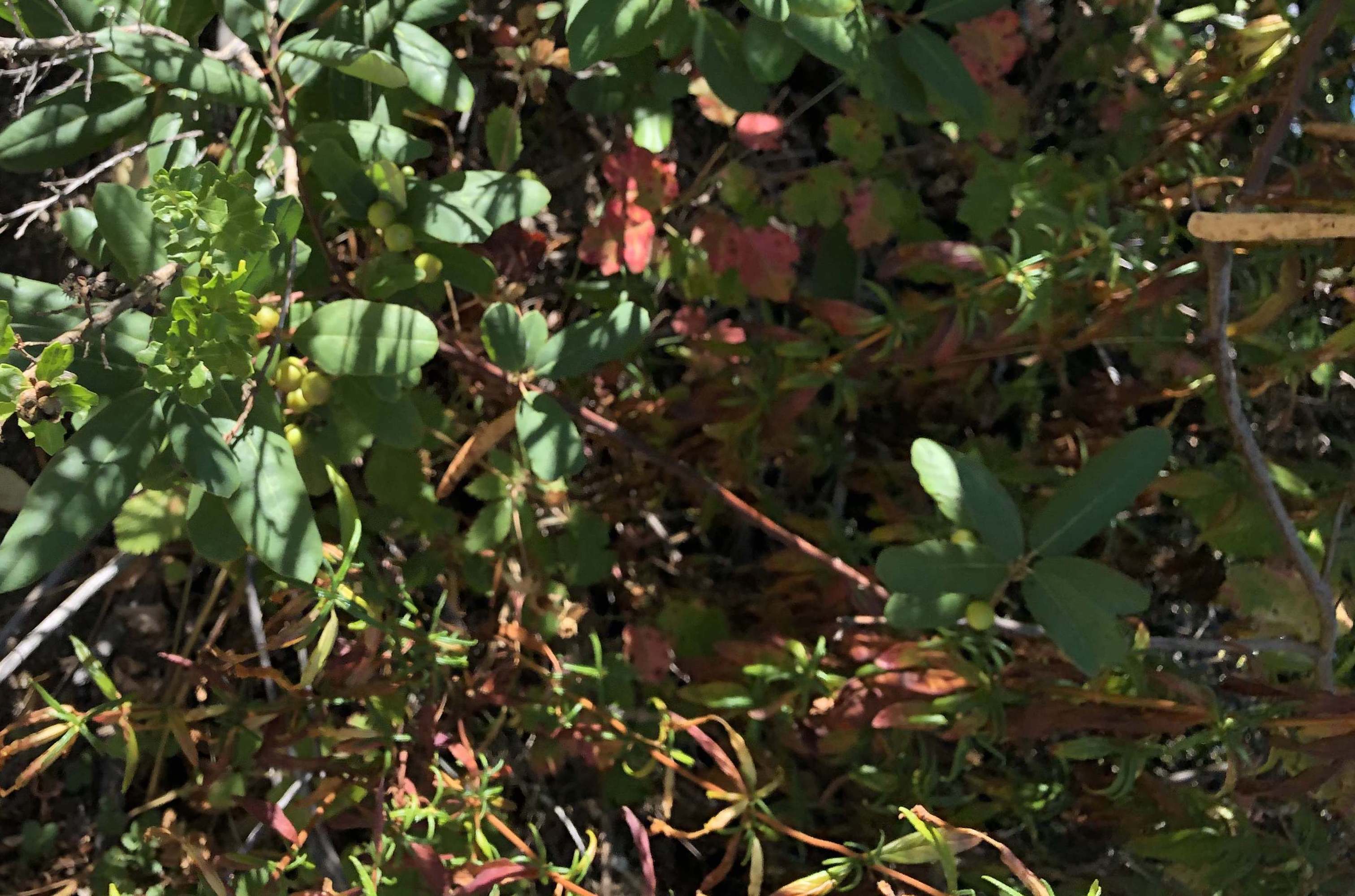
Strong red color can be indicative of poison oak but also a strong false positive.
Training Augmentation is quit helpful for this use-case. Shift and rotation especially. But I came across a moment when my validation accuracy would reach a certain point around 70% where it wouldn’t get better; but it wouldn’t get worse either. This is due to the rookie mistake of augmenting the validation data as well as the training data.
A fair comparison:

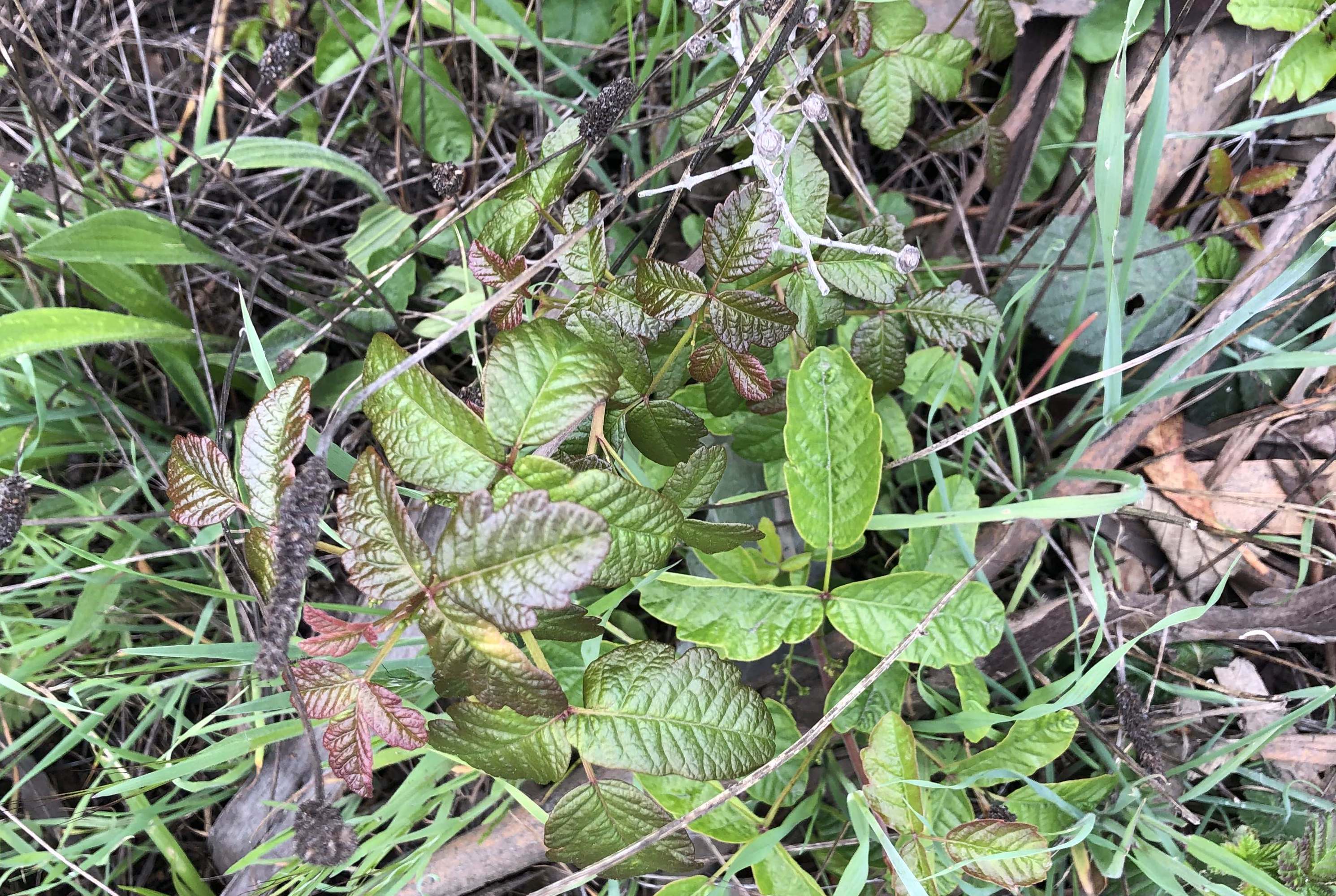
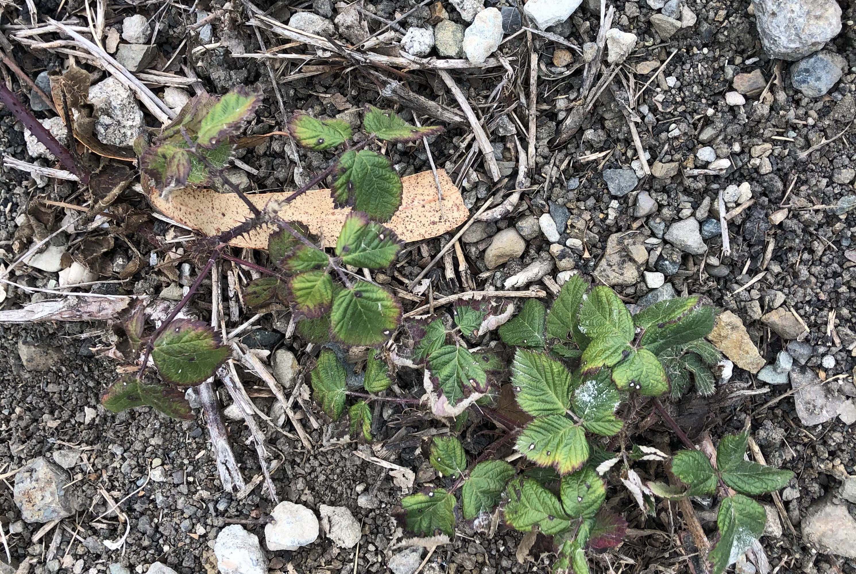
Contextual image information may often be a confounder.

Possible Next Steps:

Model experimentation with better feature extraction to take better advantage of the obvious leaf colors (edge detection, color space conversion and texture analysis, etc). Different model types such as Probabilistic Neural Network (PNN) that will accomidate a level of uncertainty among densly populated leaves in addition to be faster which is always an advantage on edge. This would be particularly useful where PNNs for classifying multiple different species of plants where the number of plants can potentially be very large and dense.

Conclusion

If you’ve gotten this far: thanks for reading!

Several training lessons were learned during the development of the Poizon Plant iOS app. I discovered that training only the last 20 layers and using Adam optimizer led to a smoother convergence and higher overall accuracy. Data augmentation techniques, such as random rotations and flips, were utilized to further improve the model’s robustness. In addition, the hyperparameters of the model were fine-tuned to achieve the best possible performance. The choice of classification task over object detection was made for practical reasons, and a goal of achieving over 90% F1 score was set. I found that focusing on high-loss images helped to understand true performance, and careful consideration was given to label the data properly. Also, the use of GPUs was important to maintain the momentum of the project. Finally, a fair comparison between images was essential to avoid contextual information as a confounder. Overall, these lessons demonstrate the importance of careful consideration and experimentation during the development of deep learning models.

I deployed the model using TensorFlow Lite, a mobile framework for running machine learning models on mobile devices. To make the model even more efficient on mobile, I used the MobileNetV2 architecture, which is designed specifically for mobile devices and has a smaller memory footprint than other CNN architectures. With the model deployed and optimized for mobile, it was ready for use in real-world applications.

References

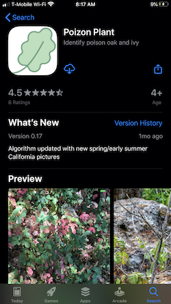
Poizon Plant iOS app (Note: the app being available to download is contingent upon free ads covering the registration cost of iOS apps. If the link is broken, it’s likely because there wasn’t enough ad revenue)